class: center, middle, inverse, title-slide # Working with factor variables --- background-image: url(https://github.com/allisonhorst/stats-illustrations/raw/master/other-stats-artwork/nominal_ordinal_binary.png) background-size: 500px background-position: 50% 90% ## Factors - A special type of variable to indicate categories - Includes both the **labels** and their **order** (i.e. numbers) - By default, text variables are stored in factors during input - Numeric categorical variables have to be converted to factors manually - `factor()` creates a new factor with specified labels ??? categorical variable = variables that have a fixed and known set of possible values --- class: yourturn # Your Turn Load a sample of data from the [General Social Survey](http://gss.norc.org/) with the following code: `data(gss_cat, package = "forcats")` Inspect the `gss_cat` object. How many variables are there? Which type does each of the variables have? Make a summary of `year`. Make `year` a factor variable: `gss_cat$year <- factor(gss_cat$year)` Compare summary of `year` to the previous result. Are there other variables that should be factors (or vice versa)? --- class: inverse, center, middle # Checking and casting <br> data types --- ## Check the data type Recall the data types in R: - logical, double, integer, character, lists, & more Checking for types: - `str` or `typeof` provide info on type - `is.XXX` (with XXX either `factor, int, numeric, logical, character, ...` ) checks for specific type ```r typeof(TRUE) ``` ``` ## [1] "logical" ``` ```r typeof("hello") ``` ``` ## [1] "character" ``` ```r is.integer(1:3) ``` ``` ## [1] TRUE ``` --- ## ⚠️ Data type coercion ⚠️ R is a dynamically typed language It will happily convert between the various types without complaint ```r c(1, "Hello") ``` ``` ## [1] "1" "Hello" ``` ```r c(FALSE, 3L) ``` ``` ## [1] 0 3 ``` ```r c(1.2, 3L) ``` ``` ## [1] 1.2 3.0 ``` --- ## Casting between types <br/> `as.XXX` casts to specific type <br/> ```r as.character(c(1, 9, 4.3, FALSE)) ``` ``` ## [1] "1" "9" "4.3" "0" ``` ```r as.numeric(c(TRUE, FALSE, FALSE)) ``` ``` ## [1] 1 0 0 ``` ```r fruits <- factor(c("apple", "banana", "orange")) as.numeric(fruits) ``` ``` ## [1] 1 2 3 ``` --- ## Casting between types  <br/> ⚠️ `as.numeric` applied to a factor retrieves *order* of labels, not labels, even if those could be interpreted as numbers. To get the labels of a factor as numbers, first cast to character and then to a number. ```r as.numeric(factor(c(4,6,1,4,7))) ``` ``` ## [1] 2 3 1 2 4 ``` --- class: inverse, center, middle # working with factor variables --- ## Levels of factor variables Use `levels(x)` to check the levels of factor variable `x` in their current order ```r levels(gss_cat$race) ``` ``` ## [1] "Other" "Black" "White" "Not applicable" ``` <br/> Use `summary(x)` to see order of the levels with counts for each level ```r summary(gss_cat$race) ``` ``` ## Other Black White Not applicable ## 1959 3129 16395 0 ``` `dplyr::count()` will also work but more on this next week... ```r gss_cat %>% count(race) ``` ``` ## # A tibble: 3 x 2 ## race n ## <fct> <int> ## 1 Other 1959 ## 2 Black 3129 ## 3 White 16395 ``` --- ## ⚠️ factors in bar charts ⚠️ A barchart can also provide us with a quick summary *provided* the <br> levels have values. .pull-left[ ```r ggplot(gss_cat, aes(race)) + geom_bar() ``` 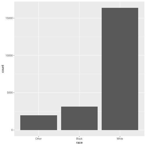<!-- --> ] .pull-right[ ```r ggplot(gss_cat, aes(race)) + geom_bar() + scale_x_discrete(drop = FALSE) ``` 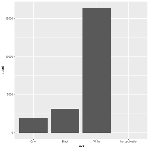<!-- --> ] --- ## ⚠️ factors in boxplots ⚠️ boxplots in ggplot2 only work properly if the x variable is a character variable or a factor: ```r twoyear <- dplyr::filter(gss_cat, year %in% c(2000, 2014)) ``` .pull-left[ ```r ggplot(data = twoyear, aes(x = year, y = tvhours)) + geom_boxplot() ``` 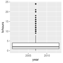<!-- --> ] .pull-right[ ```r ggplot(data = twoyear, aes(x = factor(year), y = tvhours)) + geom_boxplot() ``` 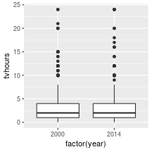<!-- --> ] --- class: inverse, center, middle # Changing the order <br>of the levels --- background-image: url(https://d33wubrfki0l68.cloudfront.net/cd4a81fe4e2b6bf9ea7af524faf5f8c9db039edb/5c672/images/hex-forcats.png) background-size: 120px background-position: 94% 5% ## Changing the order Factor variables often have to be re-ordered for ease of comparisons - We can manually specify the order of the levels by explicitly <br> listing them, see `help(factor)` - We can make the order of the levels in one variable dependent on the summary statistic of another variable - the `forcats` package (part of the `tidyverse` ⚠️ but not automatically loaded!) contains many functions to make this easier and less error-prone 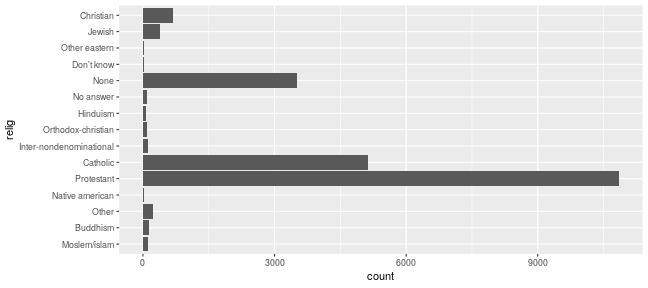<!-- --> --- ## Reordering factor levels - <br>the manual way ```r levels(gss_cat$relig) ``` ``` ## [1] "Moslem/islam" "Buddhism" "Other" ## [4] "Not applicable" "Native american" "Protestant" ## [7] "Catholic" "Inter-nondenominational" "Orthodox-christian" ## [10] "Hinduism" "No answer" "None" ## [13] "Don't know" "Other eastern" "Jewish" ## [16] "Christian" ``` manually (⚠️ extremely sensitive to typos): ```r levels(factor(gss_cat$relig, levels=c("Moslem/islam", "Hinduism", "Buddhism", "Other eastern", "Jewish", "Christian", "Orthodox-christian", "Catholic", "Protestant", "Inter-nondenominational", "Native american", "Other", "None", "No answer", "Don't know", "Not applicable"))) ``` ``` ## [1] "Moslem/islam" "Hinduism" "Buddhism" ## [4] "Other eastern" "Jewish" "Christian" ## [7] "Orthodox-christian" "Catholic" "Protestant" ## [10] "Inter-nondenominational" "Native american" "Other" ## [13] "None" "No answer" "Don't know" ## [16] "Not applicable" ``` --- background-image: url(https://d33wubrfki0l68.cloudfront.net/cd4a81fe4e2b6bf9ea7af524faf5f8c9db039edb/5c672/images/hex-forcats.png) background-size: 120px background-position: 94% 5% ## Reordering factor levels - <br> by frequency Use the function `fct_infreq()` from the `forcats` package to order the <br>categorical variable `relig` by its frequency. ```r library(forcats) ggplot(gss_cat, aes(x = fct_infreq(relig))) + geom_bar() + coord_flip() ``` 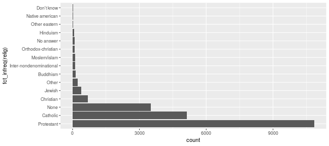<!-- --> --- ## Reordering factor levels - <br>using another variable Base R option: `reorder(factor, numbers, function)` reorder levels in factor by values in `numbers`. Use the argument `function` to summarise (average is used by default). ```r levels(reorder(gss_cat$relig, gss_cat$tvhours, na.rm=TRUE)) ``` ``` ## [1] "Other eastern" "Hinduism" "Buddhism" ## [4] "Orthodox-christian" "Moslem/islam" "Jewish" ## [7] "None" "No answer" "Other" ## [10] "Christian" "Inter-nondenominational" "Catholic" ## [13] "Protestant" "Native american" "Don't know" ## [16] "Not applicable" ``` <br/> missing values in `numbers`? make sure to use parameter `na.rm=TRUE`! --- background-image: url(https://d33wubrfki0l68.cloudfront.net/cd4a81fe4e2b6bf9ea7af524faf5f8c9db039edb/5c672/images/hex-forcats.png) background-size: 120px background-position: 94% 5% ## Reordering factor levels - <br>using another variable Option using the `forcats` package: `fct_reorder(factor, numbers, function)` ```r relig_summary <- gss_cat %>% group_by(relig) %>% summarise(age = mean(age, na.rm = TRUE), tvhours = mean(tvhours, na.rm = TRUE), n = n()) ``` .pull-left[ ```r ggplot(relig_summary, aes(x = tvhours, y = relig)) + geom_point() ``` 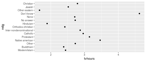<!-- --> ] .pull-right[ ```r ggplot(relig_summary, aes(x = tvhours, y = fct_reorder(relig, tvhours))) + geom_point() ``` 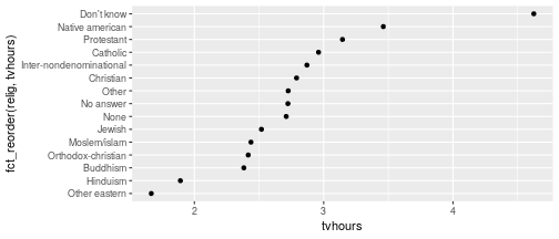<!-- --> ] --- class: yourturn .center[ # Your turn ] For this your turn use the `fbi` object: `fbi <- read.csv("https://raw.githubusercontent.com/Stat480-at-ISU/materials-2020/master/02_r-intro/data/fbi.csv")` 1. Introduce a rate of the number of reported offenses by population into the `fbi` data. You could use the *Ames standard* to make values comparable to a city of the size of Ames (population ~70,000). 2. Plot boxplots of crime rates by different types of crime. How can you make axis text legible? 3. Reorder the boxplots of crime rates, such that the boxplots are ordered by their medians. 4. For one type of crime (subset!) plot boxplots of rates by state, reorder boxplots by median crime rates --- class: inverse, center, middle # Changing the values <br> of the levels --- ## Changing Levels' names - <br> using base R ```r levels(gss_cat$partyid) ``` ``` ## [1] "No answer" "Don't know" "Other party" ## [4] "Strong republican" "Not str republican" "Ind,near rep" ## [7] "Independent" "Ind,near dem" "Not str democrat" ## [10] "Strong democrat" ``` ```r levels(gss_cat$partyid)[2] <- "Not sure" levels(gss_cat$partyid) ``` ``` ## [1] "No answer" "Not sure" "Other party" ## [4] "Strong republican" "Not str republican" "Ind,near rep" ## [7] "Independent" "Ind,near dem" "Not str democrat" ## [10] "Strong democrat" ``` --- ## Changing Levels' names - <br> using forcats The most general and powerful tool is `fct_recode()` - can recode, or change, the value of each level - levels not mentioned are left as is ```r levels(gss_cat$partyid) ``` ``` ## [1] "No answer" "Not sure" "Other party" ## [4] "Strong republican" "Not str republican" "Ind,near rep" ## [7] "Independent" "Ind,near dem" "Not str democrat" ## [10] "Strong democrat" ``` ```r partyid2 = fct_recode(gss_cat$partyid, "Republican, strong" = "Strong republican", "Republican, weak" = "Not str republican", "Independent, near rep" = "Ind,near rep", "Independent, near dem" = "Ind,near dem", "Democrat, weak" = "Not str democrat", "Democrat, strong" = "Strong democrat" ) levels(partyid2) ``` ``` ## [1] "No answer" "Not sure" "Other party" ## [4] "Republican, strong" "Republican, weak" "Independent, near rep" ## [7] "Independent" "Independent, near dem" "Democrat, weak" ## [10] "Democrat, strong" ``` --- ## Lump levels together If you want to collapse a lot of levels, `fct_collapse()` is a useful variant of `fct_recode()`. For each new variable, you can provide a vector of old levels: ```r partyid2 = fct_collapse(gss_cat$partyid, other = c("No answer", "Don't know", "Other party"), rep = c("Strong republican", "Not str republican"), ind = c("Ind,near rep", "Independent", "Ind,near dem"), dem = c("Not str democrat", "Strong democrat")) levels(partyid2) ``` ``` ## [1] "other" "Not sure" "rep" "ind" "dem" ``` <br/> You can lump together `n` small groups with `fct_lump()` ```r relig2 = fct_lump(gss_cat$relig, n = 6) summary(relig2) ``` ``` ## Protestant Catholic None Jewish Christian Other ## 10846 5124 3523 388 689 913 ``` --- ## Resources - reference/document: https://forcats.tidyverse.org/ - Wickham & Grolemund's <a href="http://r4ds.had.co.nz/factors.html">chapter on factors</a> in *R for Data Science* - Roger Peng: [*stringsAsFactors: An unauthorized biography*](http://simplystatistics.org/2015/07/24/stringsasfactors-an-unauthorized-biography/") - Thomas Lumley: <a href="http://notstatschat.tumblr.com/post/124987394001/stringsasfactors-sigh"><em>stringsAsFactors = &lt;sigh&gt;</em></a> - Artwork by [@allison_horst](https://twitter.com/allison_horst?ref_src=twsrc%5Egoogle%7Ctwcamp%5Eserp%7Ctwgr%5Eauthor)