dplyr examples: group_by and summarise

The Happy data from GSS

The General Social Survey (GSS) has been run by NORC every other year since 1972 to keep track of current opinions across the United States.

An excerpt of the GSS data called happy is available from the classdata package:

devtools::install_github("heike/classdata")

You can find a codebook with explanations for each of the variables at https://gssdataexplorer.norc.org/

A first look

library(tidyverse)
library(classdata)
data("happy", package="classdata")
happy %>% str()

## 'data.frame':    62466 obs. of  11 variables:
##  $ happy   : Factor w/ 3 levels "not too happy",..: 1 1 2 1 2 2 1 1 2 2 ...
##  $ year    : int  1972 1972 1972 1972 1972 1972 1972 1972 1972 1972 ...
##  $ age     : num  23 70 48 27 61 26 28 27 21 30 ...
##  $ sex     : Factor w/ 2 levels "female","male": 1 2 1 1 1 2 2 2 1 1 ...
##  $ marital : Factor w/ 5 levels "never married",..: 1 3 3 3 3 1 4 1 1 3 ...
##  $ degree  : Factor w/ 5 levels "lt high school",..: 4 1 2 4 2 2 2 4 2 2 ...
##  $ finrela : Factor w/ 5 levels "far below average",..: 3 4 3 3 4 4 4 3 3 2 ...
##  $ health  : Factor w/ 4 levels "poor","fair",..: 3 2 4 3 3 3 4 3 4 2 ...
##  $ polviews: Factor w/ 7 levels "extrmly conservative",..: NA NA NA NA NA NA NA NA NA NA ...
##  $ partyid : Factor w/ 8 levels "strong republican",..: 5 6 4 6 7 5 5 5 7 7 ...
##  $ wtssall : num  0.445 0.889 0.889 0.889 0.889 ...

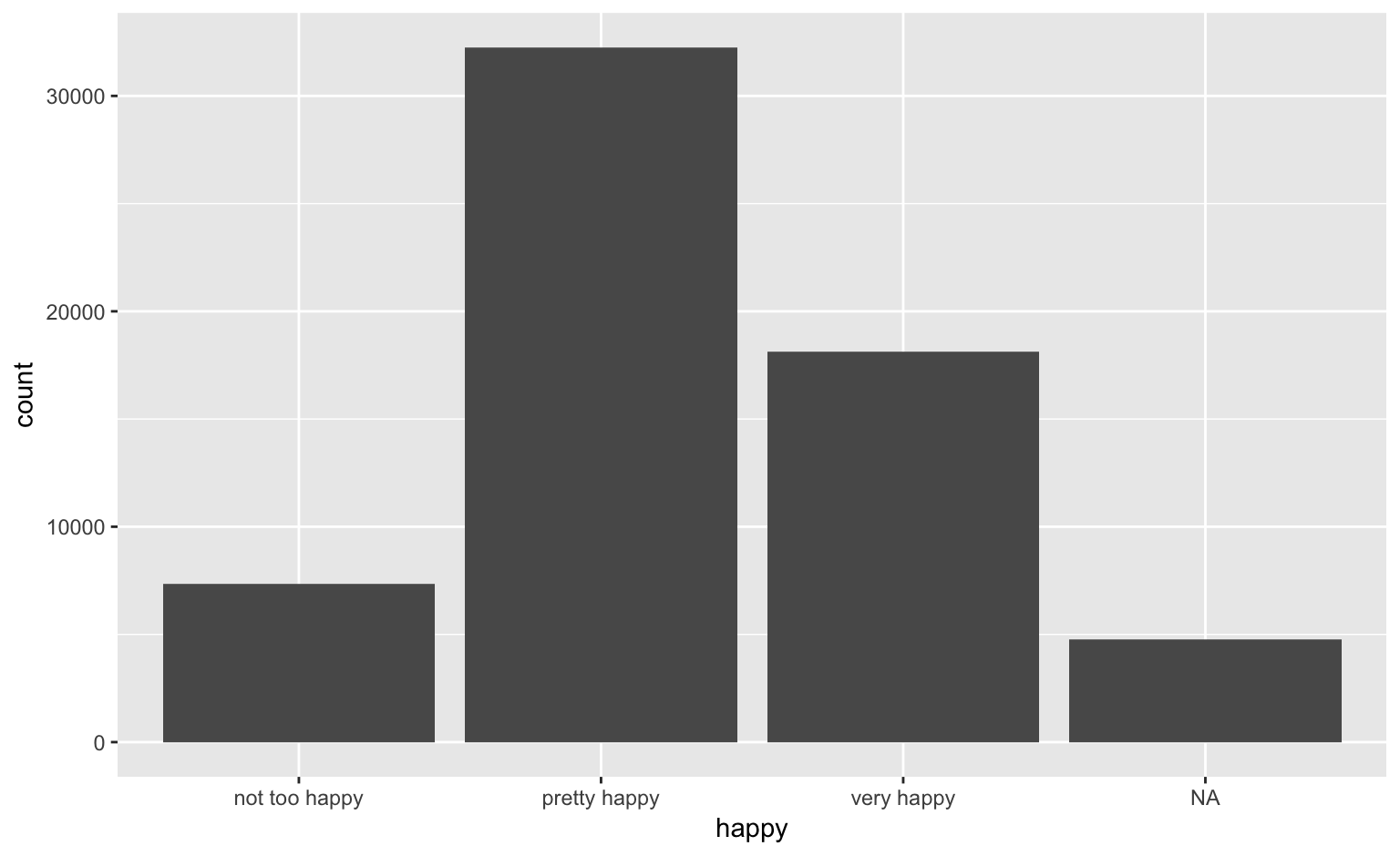
The variable `HAPPY`

happy %>% 
  ggplot(aes(x = happy)) + geom_bar()

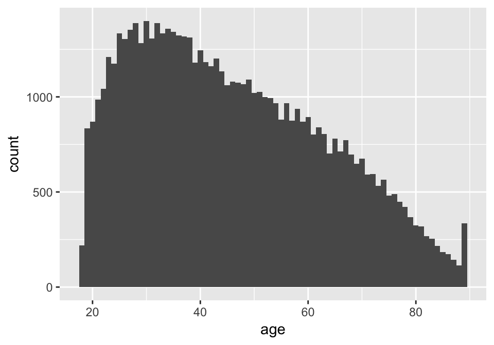
The variable `age`

happy %>% ggplot(aes(x = age)) + geom_histogram(binwidth=1)

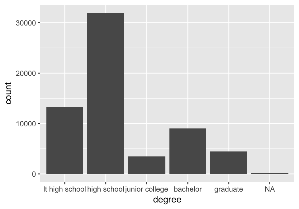
The variable `degree`

happy %>% ggplot(aes(x = degree)) + geom_bar()

Summarising Happiness

Use scores for happy factor to summarise overall happiness level, i.e. not too happy = 1, pretty happy = 2, and very happy = 3

happy %>% summarise(
  m.happy = mean(as.numeric(happy), na.rm=TRUE)
  )

##    m.happy
## 1 2.186969

happy %>% group_by(sex) %>% summarise(
  m.happy = mean(as.numeric(happy), na.rm=TRUE)
  )

## # A tibble: 2 x 2
##   sex    m.happy
##   <fct>    <dbl>
## 1 female    2.19
## 2 male      2.18

Your turn: group_by and summarise

For this your turn use the happy data from the classdata package

How do average happiness levels change over age?
Are Republicans or Democrats happier? Compare average happiness levels over partyid.
How are financial relations associated with average happiness levels? Is this association different for men and women?
Find a plot that shows the differences for each one of the summaries.

Your turn: asking questions

For this your turn use the happy data from the classdata package

Investigate what other variable(s) might be associated with happiness. Plot it.
Submit your code in Canvas for one point of extra credit.

Helper functions (1)

n() provides the number of rows of a subset:

happy %>% group_by(sex) %>% summarise(n = n())

## # A tibble: 2 x 2
##   sex        n
##   <fct>  <int>
## 1 female 34904
## 2 male   27562

tally() is a combination of summarise and n

happy %>% group_by(sex) %>% tally()

## # A tibble: 2 x 2
##   sex        n
##   <fct>  <int>
## 1 female 34904
## 2 male   27562

Helper functions (2)

count() is a further shortcut of group_by and tally:

happy %>% count(sex, degree)

## # A tibble: 12 x 3
##    sex    degree             n
##    <fct>  <fct>          <int>
##  1 female lt high school  7500
##  2 female high school    18419
##  3 female junior college  2047
##  4 female bachelor        4731
##  5 female graduate        2112
##  6 female <NA>              95
##  7 male   lt high school  5825
##  8 male   high school    13598
##  9 male   junior college  1425
## 10 male   bachelor        4279
## 11 male   graduate        2357
## 12 male   <NA>              78

group_by and summarise